Day 1

Materials

Slides
Code
Lab 1 - Deploy Quarto with GHA

Based on the book by Alex Gold “DevOps for Data Science”

We deployed a basic Quarto website at Github pages and POSIT Connect (mutiple bugs and failures) using github actions.

Import

penguin_sum <- penguins %>%
  group_by(island, year) %>%
  summarize(mean_body_mass_g = mean(body_mass_g, na.rm = TRUE)) %>% 
  ungroup()

Table

palette <- paletteer::paletteer_d("ggsci::teal_material", n = 3) %>%
  as.character()

penguin_sum %>% 
  gt() %>% 
  cols_label(
    mean_body_mass_g = "Mean Body Mass (g)"
    ) %>% 
  tab_header(
    title = md("**Mean body mass of penguins on different islands**"),
    subtitle = "2007-2009"
    ) %>% 
  data_color(
    columns = "island",
    colors = scales::col_factor(
      as.character(palette),
      domain = NULL
    )
  )

island	year	Mean Body Mass (g)
Mean body mass of penguins on different islands
2007-2009
Biscoe	2007	4740.909
Biscoe	2008	4628.125
Biscoe	2009	4792.797
Dream	2007	3684.239
Dream	2008	3779.412
Dream	2009	3691.477
Torgersen	2007	3763.158
Torgersen	2008	3856.250
Torgersen	2009	3489.062

Plot

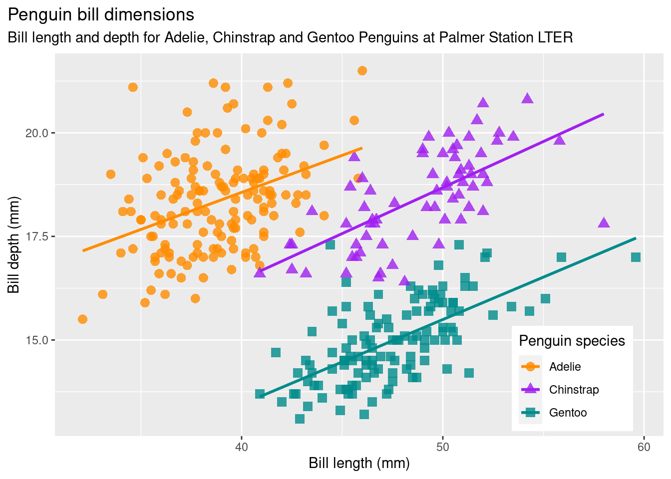
bill_len_dep <- ggplot(data = penguins,
                         aes(x = bill_length_mm,
                             y = bill_depth_mm,
                             group = species)) +
  geom_point(aes(color = species, 
                 shape = species),
             size = 3,
             alpha = 0.8) +
  geom_smooth(method = "lm", se = FALSE, aes(color = species)) +
  scale_color_manual(values = c("darkorange","purple","cyan4")) +
  labs(title = "Penguin bill dimensions",
       subtitle = "Bill length and depth for Adelie, Chinstrap and Gentoo Penguins at Palmer Station LTER",
       x = "Bill length (mm)",
       y = "Bill depth (mm)",
       color = "Penguin species",
       shape = "Penguin species") +
  theme(legend.position = c(0.85, 0.15),
        plot.title.position = "plot",
        plot.caption = element_text(hjust = 0, face= "italic"),
        plot.caption.position = "plot")

bill_len_dep